# install.packages('devtools')
# devtools::install_github('haven-jeon/KoNLP')Digital literacy in STEM special education curriculum of South Korea using descriptive statistics and natural language processing
Install R packages
Load R packages
suppressPackageStartupMessages({
  library(readxl)
  library(openxlsx)
  library(officer)
  library(flextable)
  library(tidyr)
  library(magrittr)
  library(tidyverse)
  library(purrr)
  library(dplyr)
  library(tidyr)
  library(stringr)
  library(KoNLP)
  library(tidytext)
  library(plotly)
  library(ggplot2)
  library(DT)
  library(scales)
})
Code
data <- read_excel("data/data.xlsx")

data <- data %>% mutate(across(c(type, subject, construct, coding1, coding2), as.factor))

data_filtered <- data %>%
  mutate(document = paste(id, "_", subject, "_", type, sep = "")) %>%
  select(document, everything()) %>%
  filter(!is.na(coding1) | !is.na(coding2))

long_data_filtered <- data_filtered %>%
  pivot_longer(
    cols = starts_with("coding"),
    names_to = "criteria",
    values_to = "coding") %>%
  filter(!is.na(coding)) %>%
  select(document, everything())

long_data_filtered <- long_data_filtered %>%
  mutate(competence = as.factor(gsub("\\..*", "", coding)))

long_data_filtered$competence <- as.factor(long_data_filtered$competence)

levels(long_data_filtered$competence) <- c("Competence 0",
                                      "Competence 1",
                                      "Competence 2",
                                      "Competence 3",
                                      "Competence 4",
                                      "Competence 5",
                                      "Competence 6")

math_filtered <- data_filtered %>%
  filter(subject == "Math")

long_data_math_filtered <- math_filtered %>%
  pivot_longer(
    cols = starts_with("coding"),
    names_to = "criteria",
    values_to = "coding") %>%
  select(document, everything())

science_filtered <- data_filtered %>%
  filter(subject == "Science")

long_data_science_filtered <- science_filtered %>%
  pivot_longer(
    cols = starts_with("coding"),
    names_to = "criteria",
    values_to = "coding") %>%
  select(document, everything())

ict_filtered <- data_filtered %>%
  filter(subject == "ICT")

long_data_ict_filtered <- ict_filtered %>%
  pivot_longer(
    cols = starts_with("coding"),
    names_to = "criteria",
    values_to = "coding") %>%
  select(document, everything())

long_data_filtered$subject <- factor(long_data_filtered$subject, levels = c("Math", "Science", "ICT"))

long_data_filtered$type <- factor(long_data_filtered$type, levels = c("Basic", "Common"))

table <- long_data_filtered %>%
  group_by(competence, coding, subject, type) %>%
  summarise(Count = n()) %>%
  group_by(subject) %>%
  mutate(Percentage = case_when(
    subject == "Math" ~ Count / 80 * 100,
    subject == "Science" ~ Count / 101 * 100,
    subject == "ICT" ~ Count / 401 * 100
  )) %>%
  mutate(Freq_Percent = paste0(Count, " (", round(Percentage, 1), "%)")) %>%
  select(-Count, -Percentage) %>%
  pivot_wider(names_from = subject, values_from = Freq_Percent, values_fill = list(Freq_Percent = "0 (0%)")) %>%
  ungroup()

table_flex <- table %>%
  flextable() %>%
  fontsize(size = 11) %>%
  merge_v(j = ~ competence) %>%
  theme_vanilla() %>%
  autofit()

table_flex
competence | coding | type | Math | Science | ICT |
|---|---|---|---|---|---|
Competence 0 | 0.1 | Basic | 7 (8.8%) | 6 (5.9%) | 35 (8.7%) |
0.1 | Common | 15 (18.8%) | 16 (15.8%) | 26 (6.5%) | |
0.2 | Basic | 5 (6.2%) | 7 (6.9%) | 31 (7.7%) | |
0.2 | Common | 5 (6.2%) | 12 (11.9%) | 24 (6%) | |
Competence 1 | 1.1 | Common | 4 (5%) | 3 (3%) | 8 (2%) |
1.1 | Basic | 0 (0%) | 0 (0%) | 12 (3%) | |
1.2 | Common | 8 (10%) | 4 (4%) | 17 (4.2%) | |
1.2 | Basic | 0 (0%) | 1 (1%) | 3 (0.7%) | |
1.3 | Common | 2 (2.5%) | 5 (5%) | 13 (3.2%) | |
1.3 | Basic | 0 (0%) | 0 (0%) | 4 (1%) | |
Competence 2 | 2.1 | Basic | 4 (5%) | 3 (3%) | 2 (0.5%) |
2.1 | Common | 3 (3.8%) | 2 (2%) | 4 (1%) | |
2.2 | Basic | 1 (1.2%) | 1 (1%) | 4 (1%) | |
2.2 | Common | 0 (0%) | 6 (5.9%) | 6 (1.5%) | |
2.3 | Common | 0 (0%) | 1 (1%) | 7 (1.7%) | |
2.3 | Basic | 0 (0%) | 0 (0%) | 6 (1.5%) | |
2.4 | Basic | 0 (0%) | 2 (2%) | 2 (0.5%) | |
2.4 | Common | 0 (0%) | 5 (5%) | 8 (2%) | |
2.5 | Common | 1 (1.2%) | 0 (0%) | 5 (1.2%) | |
2.5 | Basic | 0 (0%) | 0 (0%) | 6 (1.5%) | |
2.6 | Basic | 0 (0%) | 0 (0%) | 2 (0.5%) | |
Competence 3 | 3.1 | Basic | 0 (0%) | 1 (1%) | 2 (0.5%) |
3.3 | Common | 1 (1.2%) | 0 (0%) | 1 (0.2%) | |
3.4 | Basic | 0 (0%) | 0 (0%) | 1 (0.2%) | |
3.4 | Common | 0 (0%) | 0 (0%) | 34 (8.5%) | |
Competence 4 | 4.1 | Common | 1 (1.2%) | 1 (1%) | 1 (0.2%) |
4.1 | Basic | 0 (0%) | 0 (0%) | 2 (0.5%) | |
4.2 | Common | 0 (0%) | 1 (1%) | 1 (0.2%) | |
4.2 | Basic | 0 (0%) | 0 (0%) | 3 (0.7%) | |
4.3 | Basic | 0 (0%) | 2 (2%) | 6 (1.5%) | |
4.3 | Common | 0 (0%) | 4 (4%) | 2 (0.5%) | |
4.4 | Basic | 0 (0%) | 0 (0%) | 2 (0.5%) | |
Competence 5 | 5.1 | Basic | 1 (1.2%) | 1 (1%) | 7 (1.7%) |
5.1 | Common | 1 (1.2%) | 1 (1%) | 23 (5.7%) | |
5.2 | Basic | 6 (7.5%) | 4 (4%) | 24 (6%) | |
5.2 | Common | 4 (5%) | 0 (0%) | 1 (0.2%) | |
5.3 | Common | 3 (3.8%) | 5 (5%) | 5 (1.2%) | |
5.3 | Basic | 0 (0%) | 4 (4%) | 0 (0%) | |
5.4 | Common | 4 (5%) | 3 (3%) | 20 (5%) | |
5.4 | Basic | 0 (0%) | 0 (0%) | 13 (3.2%) | |
5.5 | Basic | 0 (0%) | 0 (0%) | 7 (1.7%) | |
5.5 | Common | 0 (0%) | 0 (0%) | 14 (3.5%) | |
Competence 6 | 6.1 | Basic | 2 (2.5%) | 0 (0%) | 4 (1%) |
6.1 | Common | 0 (0%) | 0 (0%) | 3 (0.7%) | |
6.2 | Basic | 2 (2.5%) | 0 (0%) | 0 (0%) |
Code
# doc <- read_docx()
#
# doc <- doc %>%
#   body_add_par("Frequency Table", style = "heading 1")
#
# doc <- doc %>%
#   body_add_flextable(table_flex)
#
# print(doc, target = "results/frequency_table.docx")
Highest Term Frequency-Inverse Document Frequency (TF-IDF) Words
Code
# Remove specific patterns from a text column.
rm_patterns <- function(data, text_col, ...) {
    homepage <- "(HTTP(S)?://)?([A-Z0-9]+(-?[A-Z0-9])*\\.)+[A-Z0-9]{2,}(/\\S*)?"
    date <- "(19|20)?\\d{2}[-/.][0-3]?\\d[-/.][0-3]?\\d"
    phone <- "0\\d{1,2}[- ]?\\d{2,4}[- ]?\\d{4}"
    email <- "[A-Z0-9.-]+@[A-Z0-9.-]+"
    hangule <- "[ㄱ-ㅎㅏ-ㅣ]+"
    punctuation <- "[:punct:]"
    text_p <- "[^가-힣A-Z0-9]"

    cleaned_data <- data %>%
        mutate(
            processed_text = !!sym(text_col) %>%
                str_remove_all(homepage) %>%
                str_remove_all(date) %>%
                str_remove_all(phone) %>%
                str_remove_all(email) %>%
                str_remove_all(hangule) %>%
                str_replace_all(punctuation, " ") %>%
                str_replace_all(text_p, " ") %>%
                str_squish()
        )

    return(cleaned_data)
}

# Extract morphemes (noun and verb families).
extract_pos <- function(data, text_col) {
    pos_init <- data %>%
        unnest_tokens(pos_init, text_col, token = SimplePos09) %>%
        mutate(pos_n = row_number())

    noun <- pos_init %>%
        filter(str_detect(pos_init, "/n")) %>%
        mutate(pos = str_remove(pos_init, "/.*$"))

    verb <- pos_init %>%
        filter(str_detect(pos_init, "/p")) %>%
        mutate(pos = str_replace_all(pos_init, "/.*$", "다"))

    pos_td <- bind_rows(noun, verb) %>%
        arrange(pos_n) %>%
        filter(nchar(pos) > 1) %>%
        tibble()

    return(pos_td)
}

# Remove stop words or irrelevant words.
stop_words <- c("다음", "고려한", "되다", "갖추다", "있다", "하다", "않다", "고려", "관련", "관련하", "우리", "있으", "하였", "피다", "일다", "이때", "내다", "이루다", "느끼다", "기르다", "살다", "오다", "위하다")

data_filtered$subject <- factor(data_filtered$subject, levels = c("Math", "Science", "ICT"))

data_filtered$type <- factor(data_filtered$type, levels = c("Basic", "Common"))

data_pos <- data_filtered %>%
  mutate(subject_type_id = paste(subject, type, id, sep = "_")) %>%
  rm_patterns(text_col = "unit") %>%
  extract_pos(text_col = "processed_text") %>%
  filter(!grepl("[0-9]", pos) &
           !pos %in% stop_words)

data_pos$pos <- case_when(
  data_pos$pos== "지도한" ~ "지도",
  data_pos$pos== "과학적" ~ "과학",
  data_pos$pos== "수학적" ~ "수학",
  data_pos$pos== "학생들이" ~ "학생",
  data_pos$pos== "학생들" ~ "학생",
  data_pos$pos== "앱을" ~ "앱",
  data_pos$pos== "환류할" ~ "환류",
  data_pos$pos== "해석한" ~ "해석",
  data_pos$pos== "느끼" ~ "느끼다",
  data_pos$pos== "기울" ~ "기울이다",
  data_pos$pos== "살펴보" ~ "살펴보다",
  data_pos$pos== "바탕으" ~ "바탕으로",
  data_pos$pos== "기르" ~ "기르다",
  data_pos$pos== "해결력과" ~ "해결력",
  data_pos$pos== "대푯값과" ~ "대푯값",
  data_pos$pos== "그리거" ~ "그리다",
  data_pos$pos== "문해력을" ~ "문해력",
  data_pos$pos== "연계함" ~ "연계",

  TRUE ~ as.character(data_pos$pos)
)

pos_tf_idf <- data_pos %>%
  count(id, pos, sort = TRUE) %>%
  bind_tf_idf(pos, id, n) %>%
  mutate_if(is.numeric, ~ round(., 3)) %>%
  ungroup()

pos_tf_idf_combined <- left_join(pos_tf_idf, data_filtered, by = "id", relationship = "many-to-many")

pos_tf_idf_combined_subject <- pos_tf_idf_combined %>%
  select(subject, competence, pos, tf_idf) %>%
  group_by(subject) %>%
  arrange(desc(tf_idf)) %>%
  top_n(20, tf_idf) %>%
  ungroup()

# write.xlsx(pos_tf_idf_combined_subject, "results/pos_tf_idf_combined_subject.xlsx")

pos_tf_idf_combined_subject <- read_excel("results/pos_tf_idf_combined_subject_en.xlsx")

pos_tf_idf_combined_subject$subject <- factor(pos_tf_idf_combined_subject$subject, levels = c("Math", "Science", "ICT"), ordered = TRUE)

tf_idf_subject <- pos_tf_idf_combined_subject %>%
  mutate(pos = reorder(pos, tf_idf)) %>%
  ggplot(aes(x = pos, y = tf_idf, fill = competence)) +
  coord_flip() +
  geom_col(alpha = 0.8) +
  facet_wrap(~ subject, ncol = 3, scales = "free") +
  labs(title = "",
  x = "",
  y = "tf-idf",
  fill = "Competence") +
  theme_minimal(base_size = 10) +
  theme(
  axis.line = element_line(color = "#3B3B3B", linewidth = 0.3),
  axis.ticks = element_line(color = "#3B3B3B", linewidth = 0.3),
  strip.text.x = element_text(size = 10, color = "#3B3B3B"),
  axis.text.x = element_text(size = 10, color = "#3B3B3B"),
  axis.text.y = element_text(size = 10, color = "#3B3B3B"),
  axis.title = element_text(size = 11, color = "#3B3B3B"),
  axis.title.x = element_text(margin = margin(t = 10)),
  axis.title.y = element_text(margin = margin(r = 10)),
  legend.title = element_text(size = 10, color = "#3B3B3B"),
  legend.text = element_text(size = 10, color = "#3B3B3B"),
  legend.title.align = 0.5,
  legend.position = "bottom")

  # tf_idf_subject_plot <- tf_idf_subject %>% ggplotly(width = 800, height = 700)

  tf_idf_subject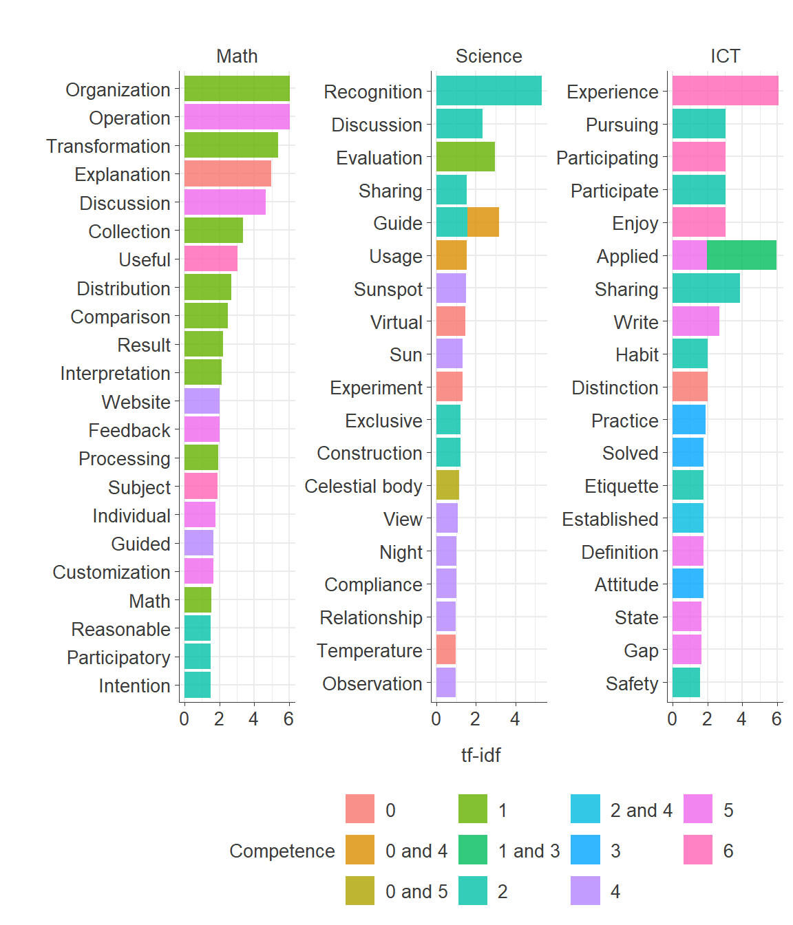
Code
ggsave("results/tf_idf_subject.png", plot = tf_idf_subject, width = 6, height = 7)Words in Basic vs. Common Mathematics Special Education Curriculum Across competences
Code
long_data_filtered$subject <- factor(long_data_filtered$subject, levels = c("Math", "Science", "ICT"))

long_data_filtered$type <- factor(long_data_filtered$type, levels = c("Basic", "Common"))

long_data_pos <- long_data_filtered %>%
  mutate(subject_type_id = paste(subject, type, id, sep = "_")) %>%
  rm_patterns(text_col = "unit") %>%
  extract_pos(text_col = "processed_text") %>%
  filter(!grepl("[0-9]", pos) &
           !pos %in% stop_words)

long_data_pos$pos <- case_when(
  long_data_pos$pos== "지도한" ~ "지도",
  long_data_pos$pos== "과학적" ~ "과학",
  long_data_pos$pos== "수학적" ~ "수학",
  long_data_pos$pos== "학생들이" ~ "학생",
  long_data_pos$pos== "학생들" ~ "학생",
  long_data_pos$pos== "앱을" ~ "앱",
  long_data_pos$pos== "환류할" ~ "환류",
  long_data_pos$pos== "해석한" ~ "해석",
  long_data_pos$pos== "느끼" ~ "느끼다",
  long_data_pos$pos== "기울" ~ "기울이다",
  long_data_pos$pos== "살펴보" ~ "살펴보다",
  long_data_pos$pos== "바탕으" ~ "바탕으로",
  long_data_pos$pos== "기르" ~ "기르다",
  long_data_pos$pos== "해결력과" ~ "해결력",
  long_data_pos$pos== "대푯값과" ~ "대푯값",
  long_data_pos$pos== "그리거" ~ "그리다",
  long_data_pos$pos== "문해력을" ~ "문해력",
  long_data_pos$pos== "연계함" ~ "연계",

  TRUE ~ as.character(long_data_pos$pos)
)

long_data_pos <- long_data_pos %>%
  mutate(competence = as.factor(gsub("\\..*", "", coding)))

sliced_math <- long_data_pos %>%
  filter(subject == "Math") %>%
  count(competence, type, pos, sort = TRUE) %>%
  pivot_wider(names_from = type, values_from = n, values_fill = 0) %>%
  mutate(n = Basic + Common) %>%
  mutate(odds_Basic = ((Basic+1)/sum(Basic+1)),
         odds_Common = ((Common+1)/sum(Common+1))) %>%
  mutate(odds_ratio = odds_Basic / odds_Common) %>%
  mutate(log_odds_ratio = log(odds_Basic / odds_Common)) %>%
  group_by(competence) %>%
  slice_max(abs(log_odds_ratio), n = 10, with_ties = FALSE) %>%
  select(competence, pos, Basic, Common, n, odds_Basic, odds_Common, odds_ratio, log_odds_ratio)

# write.xlsx(sliced_math, "results/sliced_math.xlsx")

sliced_math <- read_excel("results/sliced_math_en.xlsx")

gg_math <- sliced_math %>%
  arrange(abs(log_odds_ratio)) %>%
  mutate(pos = reorder(pos, log_odds_ratio)) %>%
  mutate_if(is.numeric, ~round(., 2)) %>%
  group_by(log_odds_ratio < 0) %>%
  ggplot(aes(pos, log_odds_ratio, fill = log_odds_ratio < 0)) +
  geom_col(alpha = 0.8) +
  scale_y_continuous(labels = label_number(accuracy = 0.01)) +
  coord_flip() +
  facet_wrap(~ competence, ncol = 3, scales = "free") +
  theme_minimal(base_size = 12) +
  theme(
  axis.line = element_line(color = "#3B3B3B", linewidth = 0.3),
  axis.ticks = element_line(color = "#3B3B3B", linewidth = 0.3),
  strip.text.x = element_text(size = 10, color = "#3B3B3B"),
  axis.text.x = element_text(size = 10, color = "#3B3B3B"),
  axis.text.y = element_text(size = 10, color = "#3B3B3B"),
  axis.title = element_text(size = 11, color = "#3B3B3B"),
  axis.title.x = element_text(margin = margin(t = 10)),
  axis.title.y = element_text(margin = margin(r = 10)),
  legend.title = element_text(size = 10, color = "#3B3B3B"),
  legend.text = element_text(size = 10, color = "#3B3B3B"),
  legend.title.align = 0.5,
  legend.position = "none") +
  labs(
    x = "",
    y = "Log odds ratio (Basic/Common)",
    fill = ""
  )

# gg_math %>% ggplotly(width = 1500, height = 500)

gg_math 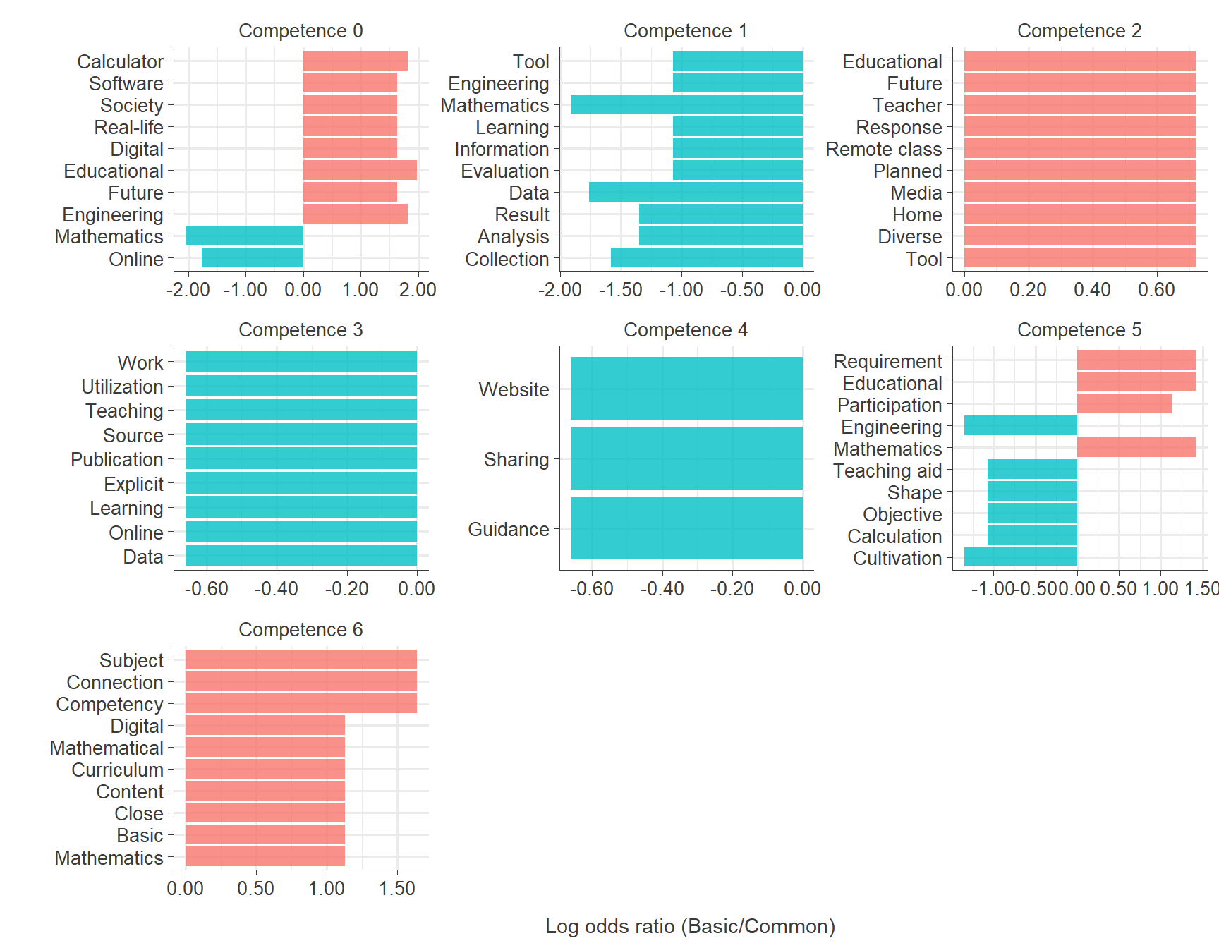
Code
ggsave("results/gg_math.png", plot = gg_math, width = 9, height = 7)Words in Basic vs. Common Science Special Education Curriculum Across competences
Code
sliced_science <- long_data_pos %>%
  filter(subject == "Science") %>%
  count(competence, type, pos, sort = TRUE) %>%
  pivot_wider(names_from = type, values_from = n, values_fill = 0) %>%
  mutate(n = Basic + Common) %>%
  mutate(odds_Basic = ((Basic+1)/sum(Basic+1)),
         odds_Common = ((Common+1)/sum(Common+1))) %>%
  mutate(odds_ratio = odds_Basic / odds_Common) %>%
  mutate(log_odds_ratio = log(odds_Basic / odds_Common)) %>%
  group_by(competence) %>%
  slice_max(abs(log_odds_ratio), n = 10, with_ties = FALSE) %>%
  select(competence, pos, Basic, Common, n, odds_Basic, odds_Common, odds_ratio, log_odds_ratio)

# write.xlsx(sliced_science, "results/sliced_science.xlsx")

sliced_science <- read_excel("results/sliced_science_en.xlsx")

gg_science <- sliced_science %>%
  arrange(abs(log_odds_ratio)) %>%
  mutate(pos = reorder(pos, log_odds_ratio)) %>%
  mutate_if(is.numeric, ~round(., 2)) %>%
  group_by(log_odds_ratio < 0) %>%
  ggplot(aes(pos, log_odds_ratio, fill = log_odds_ratio < 0)) +
  geom_col(alpha = 0.8) +
  scale_y_continuous(labels = label_number(accuracy = 0.01)) +
  coord_flip() +
  facet_wrap(~ competence, ncol = 3, scales = "free") +
  theme_minimal(base_size = 12) +
  theme(
  axis.line = element_line(color = "#3B3B3B", linewidth = 0.3),
  axis.ticks = element_line(color = "#3B3B3B", linewidth = 0.3),
  strip.text.x = element_text(size = 10, color = "#3B3B3B"),
  axis.text.x = element_text(size = 10, color = "#3B3B3B"),
  axis.text.y = element_text(size = 10, color = "#3B3B3B"),
  axis.title = element_text(size = 11, color = "#3B3B3B"),
  axis.title.x = element_text(margin = margin(t = 10)),
  axis.title.y = element_text(margin = margin(r = 10)),
  legend.title = element_text(size = 10, color = "#3B3B3B"),
  legend.text = element_text(size = 10, color = "#3B3B3B"),
  legend.title.align = 0.5,
  legend.position = "none") +
  labs(
    x = "",
    y = "Log odds ratio (Basic/Common)",
    fill = ""
  )

# gg_science %>% ggplotly(width = 1300, height = 500)

gg_science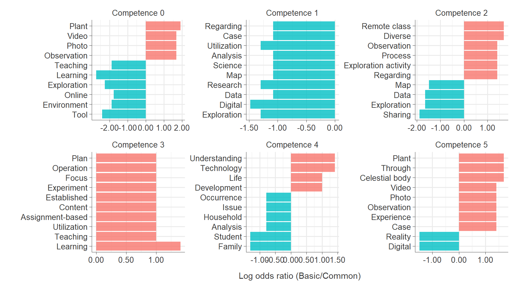
Code
ggsave("results/gg_science.png", plot = gg_science, width = 9, height = 5)Words in Basic vs. Common ICT Special Education Curriculum Across competences
Code
sliced_ict <- long_data_pos %>%
  filter(subject == "ICT") %>%
  count(competence, type, pos, sort = TRUE) %>%
  pivot_wider(names_from = type, values_from = n, values_fill = 0) %>%
  mutate(n = Basic + Common) %>%
  mutate(odds_Basic = ((Basic+1)/sum(Basic+1)),
         odds_Common = ((Common+1)/sum(Common+1))) %>%
  mutate(odds_ratio = odds_Basic / odds_Common) %>%
  mutate(log_odds_ratio = log(odds_Basic / odds_Common)) %>%
  group_by(competence) %>%
  slice_max(abs(log_odds_ratio), n = 10, with_ties = FALSE) %>%
  select(competence, pos, Basic, Common, n, odds_Basic, odds_Common, odds_ratio, log_odds_ratio)

# write.xlsx(sliced_ict, "results/sliced_ict.xlsx")

sliced_ict <- read_excel("results/sliced_ict_en.xlsx")

gg_ict <- sliced_ict %>%
  arrange(abs(log_odds_ratio)) %>%
  mutate(pos = reorder(pos, log_odds_ratio)) %>%
  mutate_if(is.numeric, ~round(., 2)) %>%
  group_by(log_odds_ratio < 0) %>%
  ggplot(aes(pos, log_odds_ratio, fill = log_odds_ratio < 0)) +
  geom_col(alpha = 0.8) +
  scale_y_continuous(labels = label_number(accuracy = 0.01)) +
  coord_flip() +
  facet_wrap(~ competence, ncol = 3, scales = "free") +
  theme_minimal(base_size = 12) +
  theme(
  axis.line = element_line(color = "#3B3B3B", linewidth = 0.3),
  axis.ticks = element_line(color = "#3B3B3B", linewidth = 0.3),
  strip.text.x = element_text(size = 10, color = "#3B3B3B"),
  axis.text.x = element_text(size = 10, color = "#3B3B3B"),
  axis.text.y = element_text(size = 10, color = "#3B3B3B"),
  axis.title = element_text(size = 11, color = "#3B3B3B"),
  axis.title.x = element_text(margin = margin(t = 10)),
  axis.title.y = element_text(margin = margin(r = 10)),
  legend.title = element_text(size = 10, color = "#3B3B3B"),
  legend.text = element_text(size = 10, color = "#3B3B3B"),
  legend.title.align = 0.5,
  legend.position = "none") +
  labs(
    x = "",
    y = "Log odds ratio (Basic/Common)",
    fill = ""
  )

# gg_ict %>% ggplotly(width = 1800, height = 500)

  gg_ict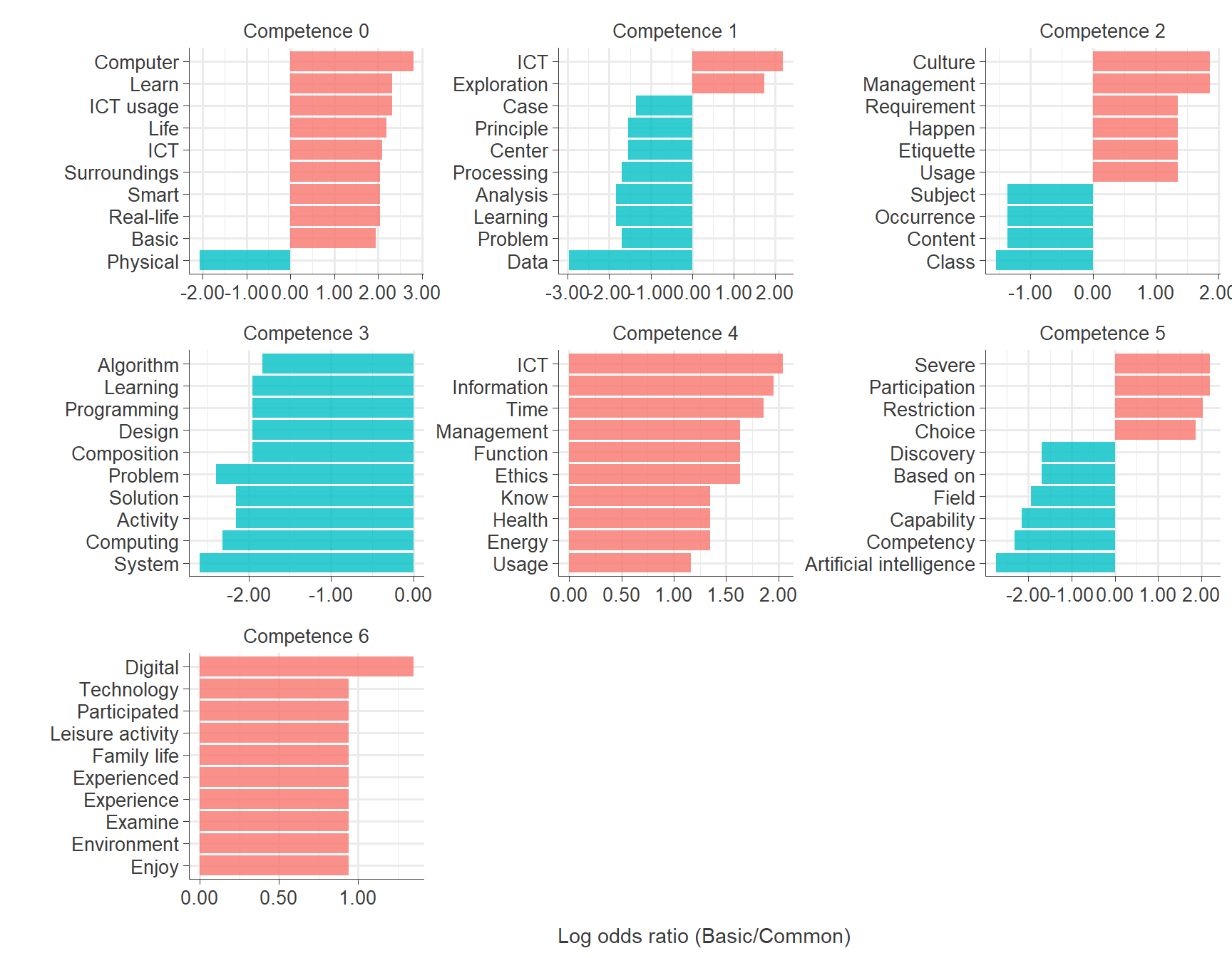
Code
ggsave("results/gg_ict.png", plot = gg_ict, width = 9, height = 7)